AI-Assisted Programming#
A Tutorial for OceanHackWeek 2023
Introduction#
Hackathons (and programming in general) involve a lot of debugging - writing code as fast as possible, running into errors, and spending hours trying to fix those errors. Many times, project teams find that they spend more time chasing errors in their code than actually focusing on the scientific work of the project!
But this workflow is about to change - with AI. Specifically, large language models (LLMs), which have shown an incredible ability to write, read, and even debug code. In the past few months, there has been a large shift toward a new workflow: AI-Assisted Programming. This workflow allows you to spend more time planning the purpose of your code while allowing a LLM to go through the drudgery of debugging.
Read about this professor’s experience implementing a birdsong classification model mere hours after attending an AI workshop at Vanderbilt!
What are LLMs?#
Before you use these tools, it’s vital to know what they are, how and why they were made, and how they get their results.
Generative AI
You may have heard this term before, as these are exactly the LLMs we will be using today. The “Generative” part of “Generative AI” (and also the “G” in “GPT”) means that the model is trained to generate text. How? By predicting the next most probably word (technically, the next token).
While we don’t know the exact training data each model used, we do know that a lot of early LLMs were trained on text available freely on the web (Wikipedia).
Keep in mind:
An LLM’ss No. 1 job is to generate text regardless of factual correctness
The Tools#
There are many LLMs available today (and more being developed each week), but we will overview three main models and what we can do with them.
ChatGPT#
The darling of the AI world, this is the most well-known LLM and gets a lot of use for writing emails and even essays. This tool does cost money (although it offers a nice free trial period).
ChatGPT offers two chat models: GPT-3.5 and GPT-4. GPT-4 is the most recent model and offers better performance, although it has a more restricted rate limit and processes less tokens than GPT-3.5.
Quick Facts
Costs money (cents per request)
No updated knowledge past Sept. 2021
Suite of coding tools with GPT-4 (Code Interpreter, plugins, API, etc.)
In this tutorial, we will be using GPT-4 with Code Interpreter.
BingGPT#
Uses a very similar model to ChatGPT, but can also use web search to aid its responses. Can only be accessed in Edge browser, but is free with a Microsoft account.
Quick Facts
Free to use (requires Edge browser)
Can access the web for answers
HuggingChat#
This free, open source chatbot uses the impressive new Llama-2 model, and is also able to search the web.
Quick Facts
Open source, free to use
Backed by new Llama-2 model
Not as widely used/tested for coding
Other Notable Tools#
GitHub Copilot: available as a plugin for VSCode and has many planned additions as part of CopilotX. Free with a school email!
Google Bard: available through Google
Poe: multiple chat models hosted on the Poe website, ability to create a custom chat bot
Prompt Engineering#
While very powerful, these AI tools are only as useful as you make them. It’s very important to understand what these models can and cannot do well, and construct your prompt accordingly.
Some strategies for prompt engineering:
Persona - tell the model to act like a programmer, scientist, teacher, etc. It will start responding like that persona.
Examples - give the model an example of the output you would like
Flipped interaction - tell the model to ask you questions until it has enough information to accomplish some task (i.e. deploying a cloud application)
Find more information about prompt engineering in this paper.
AI Assisted Workflow#
Prompt Engineer your question (specifically for coding)
Give feedback if the answer is not optimal. You can even give the model more information including details on the project, documentation of a package, and example of what you want, etc.
Run the code, and send any errors to the model
a) rinse and repeat
Use the working code. Move on to next task and start back at step (1).
Now you can get more work done, faster, and without cursing over package documentation.
Demo#
Finally, let’s demo how we can use this workflow in our coding projects. I will be taking you through a live coding session with ChatGPT 4 with Code Interpreter, but you are welcome to try this on your LLM of choice!
Note: The answers you receive from the LLM may be different from mine! Remember to use prompt engineering to steer the LLM in the direction you want to go, including any libraries or methodologies you’d like the LLM to use.
In case of technical difficulties, you can see the entire process through screenshots and code at the bottom of this notebook.
Mini Project Goal#
First, let’s establish a goal for our demonstration. Actually, we can even use ChatGPT to do this :)

So, our project goal is to predict sea surface temperature using Argo Float data
Accessing Data#
The next step of our project should be accessing our Argo SST data. Let’s see what ChatGPT can find for us:
Prompt: How do I access Argo float sea surface temperature data in Python?
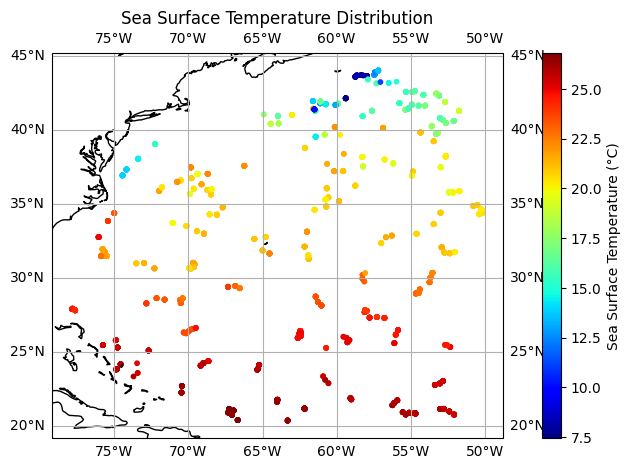
Visualizing Data#
Next, let’s plot the data on a map.
Prompt: How can I plot this data on a map?
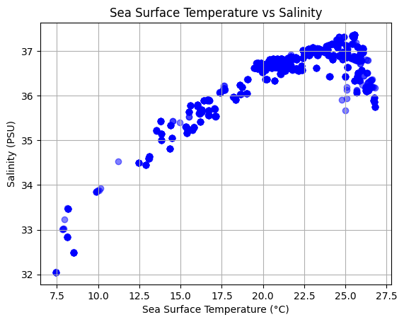
Another common visualization with SST data is SST vs Salinity. Let’s plot that relationship.
Prompt: How could I use this data to plot SST vs salinity?
Predicting SST#
Now we’ve reached the actual goal of our project: predicting SST using variables such as pressure, salinity, and lon/lat.
Prompt I want to use a machine learning model to predict sea surface temperature using other varaibles such as pressure, salinity, and lon/lat. How can I do this using the Python code generated above?
Extending this Example#
Time permitting, try to extend this example: use a more complex model, improve the model performance, add in additional data. Record your prompts and findings below.
Playground#
Now that you know how to use the tools, use the below cells to try out the AI-Assisted Workflow for your own project.
Demo via Screenshots#

# library installs if using Google Colab
#!pip install argopy xarray
from argopy import DataFetcher as ArgoDataFetcher

# Define the region: [longitude_min, longitude_max, latitude_min, latitude_max, depth_min, depth_max, time_start, time_end]
region = [-80, -50, 20, 50, 0, 10, '2021-01', '2021-02']

# Fetch data for the specified region
argo_loader = ArgoDataFetcher()
ds = argo_loader.region(region).to_xarray()

sst = ds['TEMP']
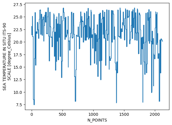
import matplotlib.pyplot as plt

sst.plot()
plt.show()

# installs for Google Colab
#!pip install cartopy
import matplotlib.pyplot as plt
import cartopy.crs as ccrs

latitude = ds['LATITUDE'].values
longitude = ds['LONGITUDE'].values
sst = ds['TEMP'].values

# Create a figure and axis with a specific projection
fig = plt.figure(figsize=(10, 5))
ax = plt.axes(projection=ccrs.PlateCarree())
ax.coastlines() # Add coastlines to the map

# Scatter plot for SST data
sc = plt.scatter(longitude, latitude, c=sst, cmap='jet', s=10, transform=ccrs.PlateCarree())
plt.colorbar(sc, label='Sea Surface Temperature (°C)')

# Add gridlines, labels, and title
ax.gridlines(draw_labels=True)
plt.title('Sea Surface Temperature Distribution')

plt.show()
/usr/local/lib/python3.10/dist-packages/cartopy/io/__init__.py:241: DownloadWarning: Downloading: https://naturalearth.s3.amazonaws.com/50m_physical/ne_50m_coastline.zip
  warnings.warn(f'Downloading: {url}', DownloadWarning)


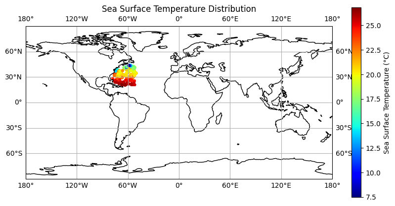
# Define the longitude and latitude boundaries for the plot
lon_min, lon_max = -180, 180
lat_min, lat_max = -90, 90

# Create a figure and axis with a specific projection
fig = plt.figure(figsize=(10, 5))
ax = plt.axes(projection=ccrs.PlateCarree())
ax.coastlines() # Add coastlines to the map

# Scatter plot for SST data
sc = plt.scatter(longitude, latitude, c=sst, cmap='jet', s=10, transform=ccrs.PlateCarree())
plt.colorbar(sc, label='Sea Surface Temperature (°C)')

# Set the map extent (zoom out to show the whole world)
ax.set_extent([lon_min, lon_max, lat_min, lat_max], crs=ccrs.PlateCarree())

# Add gridlines, labels, and title
ax.gridlines(draw_labels=True)
plt.title('Sea Surface Temperature Distribution')

plt.show()
SST vs Salinity

sst = ds['TEMP'].values
salinity = ds['PSAL'].values

import matplotlib.pyplot as plt

plt.scatter(sst, salinity, c='blue', alpha=0.5)
plt.xlabel('Sea Surface Temperature (°C)')
plt.ylabel('Salinity (PSU)')
plt.title('Sea Surface Temperature vs Salinity')
plt.grid(True)
plt.show()
Predicting

from sklearn.model_selection import train_test_split
from sklearn.linear_model import LinearRegression
from sklearn.metrics import mean_squared_error
import numpy as np

# Extract the variables
sst = ds['TEMP'].values
salinity = ds['PSAL'].values
pressure = ds['PRES'].values
latitude = ds['LATITUDE'].values
longitude = ds['LONGITUDE'].values

# Combine the features into a single array (ensure they have the same shape)
X = np.column_stack((salinity, pressure, latitude, longitude))

# Target variable (SST)
y = sst

X_train, X_test, y_train, y_test = train_test_split(X, y, test_size=0.2, random_state=42)
model = LinearRegression()
model.fit(X_train, y_train)
LinearRegression()In a Jupyter environment, please rerun this cell to show the HTML representation or trust the notebook.
On GitHub, the HTML representation is unable to render, please try loading this page with nbviewer.org.
LinearRegression()
y_pred = model.predict(X_test)
mse = mean_squared_error(y_test, y_pred)
print(f"Mean Squared Error: {mse}")
Mean Squared Error: 1.3905020768562306
from sklearn.metrics import r2_score
r2 = r2_score(y_test, y_pred)
print(f"R² Score: {r2}")
R² Score: 0.912849367517686