{
"cells": [
{
"cell_type": "code",
"execution_count": null,
"metadata": {
"slideshow": {
"slide_type": "skip"
}
},
"outputs": [],
"source": [
"from pandas.plotting import register_matplotlib_converters\n",
"\n",
"register_matplotlib_converters()\n",
"\n",
"import warnings\n",
"\n",
"warnings.filterwarnings(\"ignore\")"
]
},
{
"cell_type": "markdown",
"metadata": {
"slideshow": {
"slide_type": "slide"
}
},
"source": [
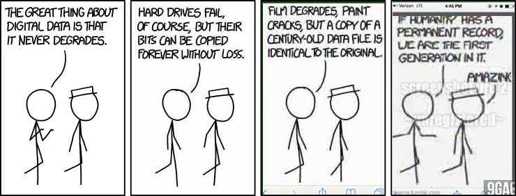
"## Data Access\n",
"\n",
"### servers, servers everywhere and not a bit to flip\n",
"\n",
"\n"
]
},
{
"cell_type": "markdown",
"metadata": {
"slideshow": {
"slide_type": "slide"
}
},
"source": [
"## whoami\n",
"\n",
"`ocefpaf` (Filipe Fernandes)\n",
"\n",
"- Physical Oceanographer\n",
"- Data Plumber\n",
"- Code Janitor\n",
"- CI babysitter\n",
"- Amazon-Dash-Button for conda-forge\n"
]
},
{
"cell_type": "markdown",
"metadata": {
"slideshow": {
"slide_type": "slide"
}
},
"source": [
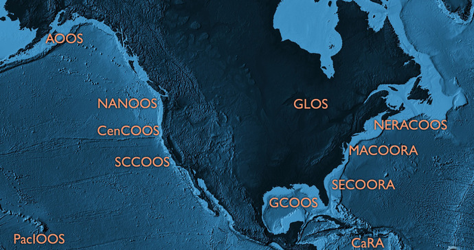
"## My day job: IOOS\n",
"\n",
"\n"
]
},
{
"cell_type": "markdown",
"metadata": {
"slideshow": {
"slide_type": "slide"
}
},
"source": [
"## Big or small we need data!\n",
"\n",
"- There are various sources: variety of servers, APIs, and web services. Just to\n",
" list a few: OPeNDAP, ERDDAP, THREDDS, ftp, http(s), S3, LAS, etc.\n",
"\n",
"\n"
]
},
{
"cell_type": "markdown",
"metadata": {
"slideshow": {
"slide_type": "slide"
}
},
"source": [
"## Feedback\n",
"\n",
"As you suffer from my tutorial on Data Access I'd love that you keep the following questions in mind so we can improve the tutorials. Should this tutorial focus on?\n",
"\n",
"- Leveraging metadata for finding data and exploring data?\n",
"- Software packages to access, slice, and dice data?\n",
"- Data sources?\n",
"- None of the above, we don't need this tutorial!"
]
},
{
"cell_type": "markdown",
"metadata": {
"slideshow": {
"slide_type": "slide"
}
},
"source": [
"## Web Services/Type of servers\n",
"\n",
"| Data Type | Web Service | Response |\n",
"| -------------------------------------- | ----------- | ----------- |\n",
"| In-situ data
(buoys, stations, etc) | OGC SOS | XML/CSV |\n",
"| Gridded data (models, satellite) | OPeNDAP | Binary |\n",
"| Raster Images | OGC WMS | GeoTIFF/PNG |\n",
"| ERDDAP | Restful API | \\* |\n",
"\n",
"- Your imagination is the limit!\n"
]
},
{
"cell_type": "markdown",
"metadata": {
"slideshow": {
"slide_type": "slide"
}
},
"source": [
"## What are we going to see in this tutorial?\n",
"\n",
"Browse and access data from:\n",
"\n",
"1. ERDDAP\n",
"2. OPeNDAP\n",
"3. ~~SOS~~\n",
"4. WMS\n",
"5. CSW and CKAN\\*\n",
"\n",
"\n",
"\\* There are many examples on CSW in [the IOOS code lab] jupyter-book (https://ioos.github.io/ioos_code_lab/content/intro.html)."
]
},
{
"cell_type": "markdown",
"metadata": {
"slideshow": {
"slide_type": "slide"
}
},
"source": [
"## 1) ERDDAP\n",
"\n",
"### Learning objectives:\n",
"\n",
"- Explore an ERDDAP server with the python interface (erddapy);\n",
"- Find a data for a time/region of interest;\n",
"- Download the data with a familiar format and create some plots.\n"
]
},
{
"cell_type": "markdown",
"metadata": {
"slideshow": {
"slide_type": "slide"
}
},
"source": [
"## What is ERDDAP?\n",
"\n",
"- Flexible outputs: .html table, ESRI .asc and .csv, .csvp, Google Earth .kml,\n",
" OPeNDAP binary, .mat, .nc, ODV .txt, .tsv, .json, and .xhtml\n",
"- RESTful API to access the data\n",
"- Standardize dates and time in the results\n",
"- Server-side searching and slicing\n"
]
},
{
"cell_type": "code",
"execution_count": null,
"metadata": {
"slideshow": {
"slide_type": "slide"
}
},
"outputs": [],
"source": [
"from erddapy import ERDDAP\n",
"\n",
"server = \"http://erddap.dataexplorer.oceanobservatories.org/erddap\"\n",
"\n",
"e = ERDDAP(server=server, protocol=\"tabledap\")"
]
},
{
"cell_type": "markdown",
"metadata": {
"slideshow": {
"slide_type": "slide"
}
},
"source": [
"### What services are available in the server?\n"
]
},
{
"cell_type": "code",
"execution_count": null,
"metadata": {
"slideshow": {
"slide_type": "fragment"
}
},
"outputs": [],
"source": [
"import pandas as pd\n",
"\n",
"df = pd.read_csv(\n",
" e.get_search_url(\n",
" response=\"csv\",\n",
" search_for=\"all\",\n",
" )\n",
")"
]
},
{
"cell_type": "code",
"execution_count": null,
"metadata": {
"slideshow": {
"slide_type": "fragment"
}
},
"outputs": [],
"source": [
"print(\n",
" f'We have {len(set(df[\"tabledap\"].dropna()))} '\n",
" f'tabledap, {len(set(df[\"griddap\"].dropna()))} '\n",
" f'griddap, and {len(set(df[\"wms\"].dropna()))} wms.'\n",
")"
]
},
{
"cell_type": "markdown",
"metadata": {
"slideshow": {
"slide_type": "slide"
}
},
"source": [
"### Let's query all the datasets that have the _standard_name_ of _sea_water_practical_salinity_.\n"
]
},
{
"cell_type": "code",
"execution_count": null,
"metadata": {
"slideshow": {
"slide_type": "fragment"
}
},
"outputs": [],
"source": [
"url = e.get_categorize_url(\n",
" categorize_by=\"standard_name\",\n",
" value=\"sea_water_practical_salinity\",\n",
" response=\"csv\",\n",
")\n",
"\n",
"df = pd.read_csv(url)\n",
"dataset_ids = df.loc[~df[\"tabledap\"].isnull(), \"Dataset ID\"].tolist()\n",
"\n",
"dataset_ids_list = \"\\n\".join(dataset_ids)\n",
"print(f\"Found {len(dataset_ids)} datasets\")"
]
},
{
"cell_type": "markdown",
"metadata": {
"slideshow": {
"slide_type": "slide"
}
},
"source": [
"### Let us narrow our search to deployments that within a lon/lat/time extent.\n"
]
},
{
"cell_type": "code",
"execution_count": null,
"metadata": {
"slideshow": {
"slide_type": "fragment"
}
},
"outputs": [],
"source": [
"from ipyleaflet import FullScreenControl, Map, Rectangle\n",
"\n",
"min_lon, max_lon = -72, -69\n",
"min_lat, max_lat = 38, 41\n",
"\n",
"rectangle = Rectangle(bounds=((min_lat, min_lon), (max_lat, max_lon)))\n",
"\n",
"m = Map(\n",
" center=((min_lat + max_lat) / 2, (min_lon + max_lon) / 2),\n",
" zoom=6,\n",
")\n",
"\n",
"m.add_layer(rectangle)\n",
"m.add_control(FullScreenControl())"
]
},
{
"cell_type": "code",
"execution_count": null,
"metadata": {
"slideshow": {
"slide_type": "slide"
}
},
"outputs": [],
"source": [
"m"
]
},
{
"cell_type": "code",
"execution_count": null,
"metadata": {
"slideshow": {
"slide_type": "fragment"
}
},
"outputs": [],
"source": [
"kw = {\n",
" \"min_time\": \"2016-07-10T00:00:00Z\",\n",
" \"max_time\": \"2017-02-10T00:00:00Z\",\n",
" \"min_lon\": min_lon,\n",
" \"max_lon\": max_lon,\n",
" \"min_lat\": min_lat,\n",
" \"max_lat\": max_lat,\n",
" \"standard_name\": \"sea_water_practical_salinity\",\n",
"}"
]
},
{
"cell_type": "code",
"execution_count": null,
"metadata": {
"scrolled": true,
"slideshow": {
"slide_type": "slide"
}
},
"outputs": [],
"source": [
"search_url = e.get_search_url(response=\"csv\", **kw)\n",
"search = pd.read_csv(search_url)\n",
"dataset_ids = search[\"Dataset ID\"].values\n",
"\n",
"dataset_ids_list = \"\\n\".join(dataset_ids)"
]
},
{
"cell_type": "code",
"execution_count": null,
"metadata": {
"slideshow": {
"slide_type": "slide"
}
},
"outputs": [],
"source": [
"print(f\"Found {len(dataset_ids)} Datasets:\\n{dataset_ids_list}\")"
]
},
{
"cell_type": "code",
"execution_count": null,
"metadata": {
"slideshow": {
"slide_type": "slide"
}
},
"outputs": [],
"source": [
"sal = \"sea_water_practical_salinity_profiler_depth_enabled\"\n",
"temp = \"sea_water_temperature_profiler_depth_enabled\"\n",
"\n",
"e.dataset_id = dataset_ids[0]\n",
"\n",
"e.variables = [\n",
" \"z\",\n",
" \"latitude\",\n",
" \"longitude\",\n",
" sal,\n",
" temp,\n",
" \"time\",\n",
"]\n",
"\n",
"url = e.get_download_url()\n",
"print(url)"
]
},
{
"cell_type": "code",
"execution_count": null,
"metadata": {
"scrolled": true,
"slideshow": {
"slide_type": "slide"
}
},
"outputs": [],
"source": [
"import pandas as pd\n",
"\n",
"df = e.to_pandas(index_col=\"time (UTC)\", parse_dates=True).dropna()\n",
"\n",
"df.head()"
]
},
{
"cell_type": "markdown",
"metadata": {
"slideshow": {
"slide_type": "slide"
}
},
"source": [
"Exercise: experiment with the `e.to_xarray()` method. Think about why/where use\n",
"one or the other?\n"
]
},
{
"cell_type": "code",
"execution_count": null,
"metadata": {
"slideshow": {
"slide_type": "slide"
}
},
"outputs": [],
"source": [
"import matplotlib.pyplot as plt\n",
"\n",
"subset = df.loc[df[\"z (m)\"] == df[\"z (m)\"].min()]\n",
"\n",
"fig, ax = plt.subplots(figsize=(13, 3.75))\n",
"subset[f\"{sal} (1e-3)\"][\"2016\"].dropna().plot(ax=ax)"
]
},
{
"cell_type": "code",
"execution_count": null,
"metadata": {
"slideshow": {
"slide_type": "skip"
}
},
"outputs": [],
"source": [
"import gsw\n",
"import numpy as np\n",
"\n",
"\n",
"def plot_ts():\n",
" fig, ax = plt.subplots(figsize=(5, 5))\n",
"\n",
" s = np.linspace(0, 42, 100)\n",
" t = np.linspace(-2, 40, 100)\n",
"\n",
" s, t = np.meshgrid(s, t)\n",
" sigma = gsw.sigma0(s, t)\n",
"\n",
" cnt = np.arange(-7, 40, 5)\n",
" cs = ax.contour(s, t, sigma, colors=\"gray\", levels=cnt)\n",
" ax.clabel(cs, fontsize=9, inline=1, fmt=\"%2i\")\n",
"\n",
" ax.set_xlabel(\"Salinity [g kg$^{-1}$]\")\n",
" ax.set_ylabel(\"Temperature [$^{\\circ}$C]\")\n",
" ax.scatter(df[f\"{sal} (1e-3)\"], df[f\"{temp} (degree_Celsius)\"], s=10, alpha=0.25)\n",
"\n",
" ax.grid(True)\n",
" ax.axis([20, 40, 4, 26])\n",
" return fig, ax"
]
},
{
"cell_type": "code",
"execution_count": null,
"metadata": {
"slideshow": {
"slide_type": "slide"
}
},
"outputs": [],
"source": [
"fig, ax = plot_ts()"
]
},
{
"cell_type": "code",
"execution_count": null,
"metadata": {
"slideshow": {
"slide_type": "slide"
}
},
"outputs": [],
"source": [
"responses = [\"mat\", \"json\", \"ncCF\", \"ncCFHeader\"]\n",
"\n",
"for response in responses:\n",
" print(f\"{e.get_download_url(response=response)}\\n\")"
]
},
{
"cell_type": "markdown",
"metadata": {
"slideshow": {
"slide_type": "slide"
}
},
"source": [
"Exercise: explore the web interface for the OOI server URL:\n",
"\n",
"http://erddap.dataexplorer.oceanobservatories.org/erddap/index.html\n",
"\n",
"or the IOOS glider dac:\n",
"\n",
"https://gliders.ioos.us/erddap\n",
"\n",
"and find a dataset of interested, download a format that you are familiar with\n",
"and plot it (using the web interface or the Python, your choice).\n"
]
},
{
"cell_type": "markdown",
"metadata": {
"slideshow": {
"slide_type": "slide"
}
},
"source": [
"## 2) OPeNDAP\n",
"\n",
"### Learning objectives:\n",
"\n",
"- Open model data from a THREDDS server via OPeNDAP with `xarray`;\n",
"- Discuss the differences with an `erddapy` request;\n",
"- Plot it using `xarray` interface.\n"
]
},
{
"cell_type": "code",
"execution_count": null,
"metadata": {
"scrolled": false,
"slideshow": {
"slide_type": "slide"
}
},
"outputs": [],
"source": [
"import cf_xarray\n",
"import xarray as xr\n",
"\n",
"url = (\n",
" \"http://tds.marine.rutgers.edu/thredds/dodsC/roms/doppio/2017_da/avg/Averages_Best\"\n",
")\n",
"ds = xr.open_dataset(url)\n",
"ds.cf"
]
},
{
"cell_type": "code",
"execution_count": null,
"metadata": {},
"outputs": [],
"source": [
"variable = \"sea_water_potential_temperature\"\n",
"time = \"2022-08-10\"\n",
"surface = -1\n",
"\n",
"selection = ds.cf[variable].sel(time=\"2022-08-10\").isel(s_rho=surface)"
]
},
{
"cell_type": "code",
"execution_count": null,
"metadata": {
"slideshow": {
"slide_type": "slide"
}
},
"outputs": [],
"source": [
"import cartopy.crs as ccrs\n",
"import matplotlib.pyplot as plt\n",
"\n",
"fig, ax = plt.subplots(\n",
" figsize=(6, 6),\n",
" subplot_kw={\"projection\": ccrs.PlateCarree()},\n",
")\n",
"\n",
"selection.plot(\n",
" ax=ax,\n",
" x=\"lon_rho\",\n",
" y=\"lat_rho\",\n",
")\n",
"\n",
"ax.coastlines()"
]
},
{
"cell_type": "markdown",
"metadata": {
"slideshow": {
"slide_type": "slide"
}
},
"source": [
"## 3) ~~SOS~~\n",
"\n",
"### Learning objectives:\n",
"\n",
"- Use searvey to obtain CO-OPS data\n"
]
},
{
"cell_type": "code",
"execution_count": null,
"metadata": {
"scrolled": true,
"slideshow": {
"slide_type": "slide"
}
},
"outputs": [],
"source": [
"import shapely\n",
"from searvey import coops\n",
"\n",
"secoora = shapely.geometry.box(-87.4, 24.25, -74.7, 36.7)\n",
"df = coops.coops_stations_within_region(secoora)\n",
"df"
]
},
{
"cell_type": "code",
"execution_count": null,
"metadata": {},
"outputs": [],
"source": [
"df.loc[df[\"name\"] == \"Duck\"]"
]
},
{
"cell_type": "code",
"execution_count": null,
"metadata": {},
"outputs": [],
"source": [
"from datetime import datetime, timedelta\n",
"\n",
"from searvey.coops import COOPS_Station\n",
"\n",
"station = COOPS_Station(\"Duck\")\n",
"\n",
"ds = station.product(\n",
" \"water_level\",\n",
" start_date=datetime.today() - timedelta(15),\n",
" end_date=datetime.today(),\n",
")\n",
"\n",
"ds[\"v\"].plot()"
]
},
{
"cell_type": "markdown",
"metadata": {
"slideshow": {
"slide_type": "slide"
}
},
"source": [
"## 4) WMS\n",
"\n",
"### Learning objectives:\n",
"\n",
"- Add a WMS layer to an interactive map. (\"Hurricane viz widget.\")\n"
]
},
{
"cell_type": "code",
"execution_count": null,
"metadata": {
"slideshow": {
"slide_type": "slide"
}
},
"outputs": [],
"source": [
"from ipyleaflet import FullScreenControl, Map, WMSLayer, basemaps\n",
"from ipywidgets import SelectionSlider\n",
"from traitlets import Unicode\n",
"\n",
"time_options = [\n",
" \"13:00\",\n",
" \"13:30\",\n",
" \"14:00\",\n",
" \"14:30\",\n",
" \"15:00\",\n",
" \"15:30\",\n",
" \"16:00\",\n",
" \"16:30\",\n",
" \"17:00\",\n",
" \"17:30\",\n",
" \"18:00\",\n",
" \"18:30\",\n",
"]\n",
"\n",
"slider = SelectionSlider(description=\"Time:\", options=time_options)\n",
"\n",
"\n",
"def update_wms(change):\n",
" time_wms.time = \"2020-07-25T{}\".format(slider.value)\n",
"\n",
"\n",
"slider.observe(update_wms, \"value\")\n",
"\n",
"\n",
"class TimeWMSLayer(WMSLayer):\n",
" time = Unicode(\"\").tag(sync=True, o=True)"
]
},
{
"cell_type": "code",
"execution_count": null,
"metadata": {
"slideshow": {
"slide_type": "slide"
}
},
"outputs": [],
"source": [
"time_wms = TimeWMSLayer(\n",
" url=\"https://mesonet.agron.iastate.edu/cgi-bin/wms/nexrad/n0r-t.cgi?\",\n",
" layers=\"nexrad-n0r-wmst\",\n",
" time=\"2020-07-25T13:00:00Z\",\n",
" format=\"image/png\",\n",
" transparent=True,\n",
" attribution=\"Weather data © 2012 IEM Nexrad\",\n",
")\n",
"m = Map(basemap=basemaps.CartoDB.Positron, center=(30, -88), zoom=5)\n",
"m.add_layer(time_wms)\n",
"m.add_control(FullScreenControl())"
]
},
{
"cell_type": "code",
"execution_count": null,
"metadata": {
"slideshow": {
"slide_type": "slide"
}
},
"outputs": [],
"source": [
"m"
]
},
{
"cell_type": "code",
"execution_count": null,
"metadata": {
"slideshow": {
"slide_type": "fragment"
}
},
"outputs": [],
"source": [
"slider"
]
},
{
"cell_type": "markdown",
"metadata": {
"slideshow": {
"slide_type": "slide"
}
},
"source": [
"## 5) Catalog Service Web (CSW)\n",
"\n",
"### Is there a canonical source for data?\n"
]
},
{
"cell_type": "markdown",
"metadata": {
"slideshow": {
"slide_type": "fragment"
}
},
"source": [
"\n"
]
},
{
"cell_type": "markdown",
"metadata": {
"slideshow": {
"slide_type": "fragment"
}
},
"source": [
"Well, kind of... The closet thing is are data catalogs like the [IOOS CSW catalog](https://data.ioos.us/) or [pangeo-forge](https://pangeo-forge.readthedocs.io/en/latest/)."
]
},
{
"cell_type": "markdown",
"metadata": {
"slideshow": {
"slide_type": "slide"
}
},
"source": [
"## Catalog Service for the Web (CSW)\n",
"\n",
"- A single source to find endpoints\n",
"- Nice python interface:
`owslib.csw.CatalogueServiceWeb`\n",
"- Advanced filtering:
`owslib.fes`\n"
]
},
{
"cell_type": "markdown",
"metadata": {
"slideshow": {
"slide_type": "slide"
}
},
"source": [
"\n"
]
},
{
"cell_type": "markdown",
"metadata": {
"slideshow": {
"slide_type": "slide"
}
},
"source": [
"## For more complex examples on how to find data in the catalog please check the IOOS code gallery:\n",
"\n",
"[https://ioos.github.io/ioos_code_lab/content/intro.html](https://ioos.github.io/ioos_code_lab/content/intro.html)\n"
]
},
{
"cell_type": "markdown",
"metadata": {
"slideshow": {
"slide_type": "slide"
}
},
"source": [
"## Where to find data?\n"
]
},
{
"cell_type": "markdown",
"metadata": {
"slideshow": {
"slide_type": "fragment"
}
},
"source": [
"Curated list of ERDDAP servers:\n",
"https://github.com/IrishMarineInstitute/awesome-erddap\n",
"\n",
"Environmental Data Service (EDS) model viewer: https://eds.ioos.us\n",
"\n",
"Exploring THREDDS servers: https://unidata.github.io/siphon/latest\n"
]
},
{
"cell_type": "markdown",
"metadata": {
"slideshow": {
"slide_type": "slide"
}
},
"source": [
"## Extras: how does this all work?\n"
]
},
{
"cell_type": "markdown",
"metadata": {
"slideshow": {
"slide_type": "fragment"
}
},
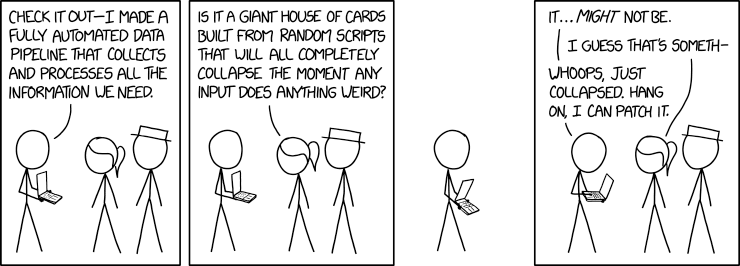
"source": [
"## Standards!\n",
"\n",
"\n"
]
},
{
"cell_type": "markdown",
"metadata": {
"slideshow": {
"slide_type": "slide"
}
},
"source": [
"## Bad example\n"
]
},
{
"cell_type": "code",
"execution_count": null,
"metadata": {
"slideshow": {
"slide_type": "fragment"
}
},
"outputs": [],
"source": [
"import cftime\n",
"import nc_time_axis\n",
"from netCDF4 import Dataset\n",
"\n",
"url = \"http://goosbrasil.org:8080/pirata/B19s34w.nc\"\n",
"nc = Dataset(url)\n",
"\n",
"temp = nc[\"temperature\"][:]\n",
"times = nc[\"time\"]\n",
"temp[temp <= -9999] = np.NaN\n",
"t = cftime.num2date(times[:], times.units, calendar=times.calendar)"
]
},
{
"cell_type": "code",
"execution_count": null,
"metadata": {},
"outputs": [],
"source": [
"mask = (t >= datetime(2008, 1, 1)) & (t <= datetime(2008, 12, 31))"
]
},
{
"cell_type": "code",
"execution_count": null,
"metadata": {
"slideshow": {
"slide_type": "slide"
}
},
"outputs": [],
"source": [
"fig, ax = plt.subplots()\n",
"ax.plot(t[mask], temp[:, 0][mask], \".\")"
]
},
{
"cell_type": "markdown",
"metadata": {
"slideshow": {
"slide_type": "slide"
}
},
"source": [
"## Good example\n"
]
},
{
"cell_type": "code",
"execution_count": null,
"metadata": {
"slideshow": {
"slide_type": "fragment"
}
},
"outputs": [],
"source": [
"import xarray as xr\n",
"\n",
"ds = xr.open_dataset(url)\n",
"temp = ds[\"temperature\"]"
]
},
{
"cell_type": "code",
"execution_count": null,
"metadata": {
"slideshow": {
"slide_type": "slide"
}
},
"outputs": [],
"source": [
"temp.sel(depth_t=1.0, time=\"2008\").plot()"
]
}
],
"metadata": {
"celltoolbar": "Slideshow",
"kernelspec": {
"display_name": "Python 3 (ipykernel)",
"language": "python",
"name": "python3"
},
"language_info": {
"codemirror_mode": {
"name": "ipython",
"version": 3
},
"file_extension": ".py",
"mimetype": "text/x-python",
"name": "python",
"nbconvert_exporter": "python",
"pygments_lexer": "ipython3",
"version": "3.9.13"
},
"livereveal": {
"auto_select": "none",
"footer": " ",
"header": "",
"start_slideshow_at": "selected"
}
},
"nbformat": 4,
"nbformat_minor": 4
}